Interpolation et Approximation de courbes
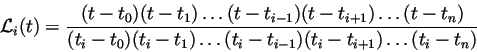
Pour  points on fabrique un polynôme de degré
  de la façon
suivante :
de la façon
suivante :
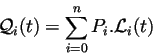
Alors le polynôme dont la représentation passe par les points est :
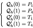
On veut définir une courbe de degré 3 passant par deux points et dont
les tangentes en ce points sont données. Soit :
On cherche à exprimer la courbe
 .
.
 étant la matrice des contraintes. Ces contraintes peuvent s'écrirent sous
la forme
étant la matrice des contraintes. Ces contraintes peuvent s'écrirent sous
la forme
 .
.  étant le vecteur de
contrôle géométrique égal à :
étant le vecteur de
contrôle géométrique égal à :
 . On a
donc :
. On a
donc :
et
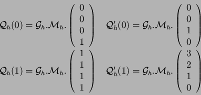
On a donc les quatres équations suivantes à résoudre :
ce que l'on peut écrire :
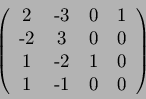
avec
On a donc :
donc
Ainsi :
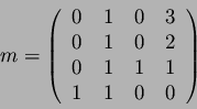
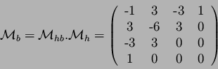
La contrainte géométrique est cette fois définie par quatre points et
non plus deux points et deux tangentes. On construit donc une courbe
hermitienne avec
 et
et
 . On cherche
une courbe du troisième degré ayant un bon comportement, notamment une
vitesse uniforme sur la ligne engendrée par quatre points alignés.
Prenons
. On cherche
une courbe du troisième degré ayant un bon comportement, notamment une
vitesse uniforme sur la ligne engendrée par quatre points alignés.
Prenons  ,
,  ,
,  et
et  . On a :
Une vitesse uniforme signifie que
 , donc :
et donc
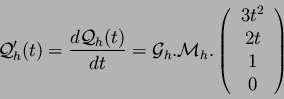
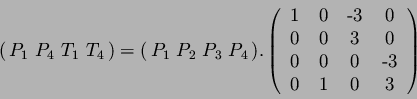
On cherche, maintenant, à exprimer la courbe sous la forme
 . On a
 , c'est-a-dire :
donc :
avec
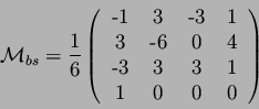
Ainsi on obtient :
On peut remarquer que
 .
La formule généralisée de la courbe de Bézier est :
.
La formule généralisée de la courbe de Bézier est :
L'inconvenient des courbes de Bézier (entre autres courbes) est que la
modification d'un seul des points influe sur l'ensemble de la courbe. On
voudrait que les points ne contrôlent la courbe que localement. On se donne
 points (
 ). Et l'on construit
  courbes cubiques :
 . Chaque courbe
  sera contrôlée par les quatre
points
sera contrôlée par les quatre
points
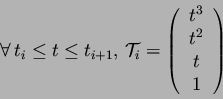
 . On cherche donc à exprimer :
La courbe
 est définie pour
 .
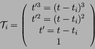
Pour des raisons de commodité on pose
.
Pour des raisons de commodité on pose  . Et l'uniformité signifie
que l'on pose que
. Et l'uniformité signifie
que l'on pose que
 .
On a :
.
On a :
Un changement de variable ( ) nous permet d'obtenir :
Jean-Baptiste Yunes
2002-01-21